Brownian Motion with 3D-Printed Microscope

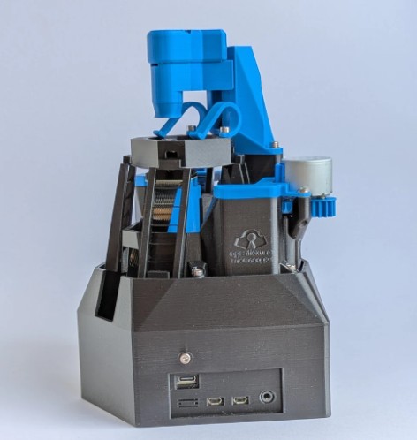
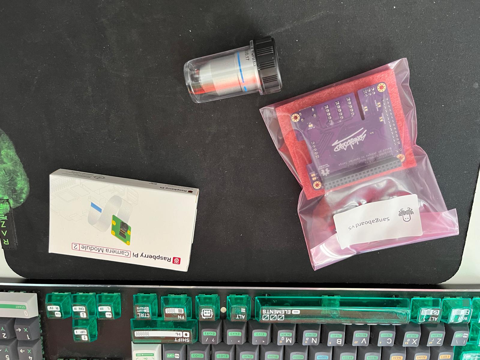
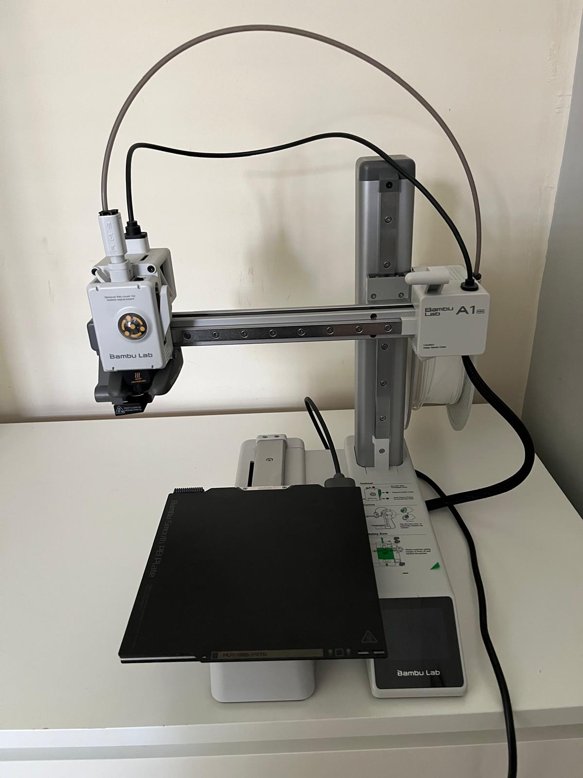
I built an openflexure microscope with printed parts, assembled the optics, and used Python to track Brownian motion of particles (micrometer scale). This page documents the build, the experiment, and my results.

3D Printing Microscopy Python
Microscope close up

Placeholder image — swap with a FINAL hero.

Project Overview

Openflexure is an open-source, 3D‑printed microscope with a flexure-based stage. I printed the components, sourced optics (from LabCrafter), and assembled the mechanism at home. The goal: capture videos of Brownian motion of different microscopic sized particles in water and analyze the diffusion using Python.

What I built

  • 3D‑printed frame, flexure stage, and optics mounts
  • Raspberry Pi camera module + LED illumination
  • Manual focus with fine Z motion

What I measured

  • Tracked bead positions (x, y) over time
  • Computed Mean Squared Displacement (MSD)
  • Estimated diffusion coefficient D

Build Notes

Here’s how I assembled the microscope. Swap the text with your own steps, tips, and photos.

  1. Print & Prep

    Step 1

    Printed parts at 0.2 mm layer height. Cleaned supports and heat‑set inserts.

  2. Stage & Optics

    Step 2

    Assembled flexure stage, mounted objective, aligned tube lens and camera.

  3. Illumination

    Step 3

    Installed LED and diffuser for bright‑field imaging.

Brownian Motion Experiment

I prepared a dilute suspension of polystyrene beads in water and recorded a video through the microscope. The bead trajectories were tracked in Python. Assuming 2D diffusion, the MSD relates to time lag Δt by MSD(Δt) = 4 D Δt, where D is the diffusion coefficient.

Python Tracking Snippet (using trackpy)
import pandas as pd
import trackpy as tp
import pims

# Load frames (e.g., mp4 converted to image sequence or using pims.Video)
frames = pims.Video('beads.mp4')

# Locate bright beads (~3 px radius)
f = tp.batch(frames, diameter=9, minmass=500)

# Link features into trajectories (search range in pixels)
linked = tp.link_df(f, search_range=10)

# Filter short trajectories
traj = tp.filter_stubs(linked, threshold=30)

# Compute mean-squared displacement (MSD)
msd = tp.emsd(traj, mpp=0.1, fps=30)  # mpp: microns per pixel, fps: frames per second
print(msd.head())

# Estimate diffusion coefficient from linear fit of MSD vs lag time

Swap mpp with your calibration (µm/pixel) and fps with your frame rate.

Recording Setup Tips
  • Use a thin sample and avoid convection—wait 1–2 minutes after sealing.
  • Record at a constant frame rate (e.g., 30 fps) and stable lighting.
  • Focus on a plane with sparse, non‑overlapping beads.

Placeholder for Brownian motion video (mp4).

Results

Upload a CSV of tracked bead centers to plot trajectories and compute MSD. Expected columns: time_s,x_um,y_um. Sampling should be uniform in time.

Data

Estimated D: µm²/s

Trajectory (x vs y)

MSD vs Δt

Note: MSD is computed across lags assuming uniform time steps; only initial lags are used for the linear fit.